

What if predictable seasonal shifts could give traders a measurable edge in correlation-based strategies this quarter?
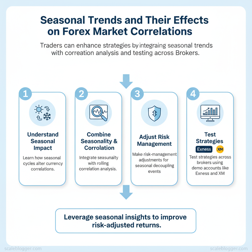
Seasonal trends often reshape forex market correlations in repeatable ways, and incorporating those patterns into portfolio construction reduces unexpected exposure during known risk periods. Traders who overlay seasonality signals with standard correlation coefficient analysis can anticipate when historically strong pairs decouple and when cross-asset relationships tighten.
This matters because currency correlation patterns drive hedge effectiveness, position sizing, and pair selection. Industry research shows momentum and carry strategies can behave differently across seasonal windows, so blending calendar-aware filters improves risk-adjusted returns. Picture a trading desk that reduces correlated EUR/USD and GBP/USD exposure each September, lowering drawdown during historically volatile windows.
Rand FX provides comparative broker tools and educational resources to test seasonally adjusted strategies in demo accounts. Use an Exness demo to validate timing rules, or try XM, HFM, or FBS for parallel testing across execution environments. Practical application of these insights spans from intraday hedging to longer-term overlay portfolios.
- How seasonal cycles historically alter major and minor currency correlations
- Methods to combine seasonality with
rolling correlationanalysis - Risk-management adjustments for seasonal decoupling events
- How to test strategies across brokers using demo accounts like Exness and XM
Compare forex brokers in South Africa: https://randfx.co.za/brokers/broker-comparison/
How Seasonal Trends are Identified in Forex Markets
Seasonal patterns in FX show up when exchange-rate behaviour repeats around the same calendar windows — quarter-ends, holiday periods, crop cycles, or central-bank meeting seasons. Traders identify these cycles by assembling long, clean historical series, applying simple rolling statistics to reveal recurring mean and volatility shifts, then validating with statistics or spectral methods to separate true seasonality from noise. Practical work begins with choosing the right data, selecting a minimum sample length to avoid overfitting, and using tests that match the signal strength: moving averages and t-tests for clear, calendar-linked effects; Fourier or wavelet analysis for subtle periodicities.
Data sources and timeframes: what to use and why
- Choose long samples: aim for at least 5–10 years of intraday/daily data to capture multiple repeats of annual cycles.
- Prefer consolidated feeds: interbank aggregators smooth out single-dealer idiosyncrasies; broker feeds capture execution-level behaviour that retail strategies will face.
- Watch update frequency: hourly/tick data expose intraday seasonal effects (e.g., month-end liquidity), daily fixes suffice for macro calendar effects.
- Mitigate biases: control for structural breaks (regime changes, major policy shifts) and survivorship bias by including delisted pairs or drilling into exchange-level logs.
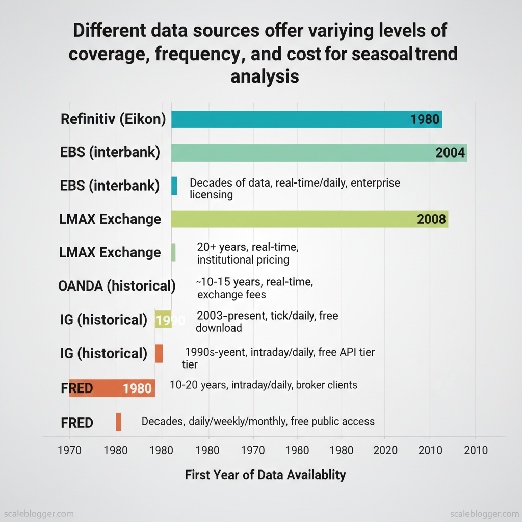
| Source | Data coverage (years) | Update frequency | Typical cost / access |
|---|---|---|---|
| Refinitiv (Eikon) | decades (1980s–present) | real-time / daily | Enterprise licensing; contact sales |
| EBS (interbank) | 20+ years | real-time | Institutional pricing; subscription |
| LMAX Exchange | ~10–15 years | real-time | Exchange fees; commercial access |
| Dukascopy historical | 2003–present | tick/daily | Free download for many pairs |
| OANDA historical rates | 1990s–present | intraday/daily | Free API tier; commercial plans |
| IG historical feed | 10–20 years | intraday/daily | Broker clients; platform access |
| Federal Reserve Economic Data (FRED) | decades (varies by series) | daily/weekly/monthly | Free public access |
| Commercial tick vendors (TickData, QuantHouse) | >20 years for major pairs | tick / intraday | Custom pricing; enterprise contracts |
Key insight: Dukascopy and FRED provide low-cost starting points for most researchers, while Refinitiv, EBS and commercial tick vendors supply the depth and cleanliness required for institutional-grade testing. Combining broker-level and interbank data reduces execution bias when validating strategies.
Statistical methods traders run (practical)
- Seasonal averages and rolling windows: compute mean returns for each calendar bucket (day-of-week, month) and compare with overall mean using
t-testor bootstrap. - Seasonal decomposition: apply
STL(seasonal-trend decomposition using Loess) to isolate seasonal component from trend and residuals. - Autocorrelation checks: plot ACF/PACF to reveal periodic lags at 5, 20, 252 days (weekly, monthly, yearly).
- Spectral analysis: use
FFTor periodogram when seasonality is not aligned to calendar dates; good for multi-frequency cyclicality. - Wavelet transforms: prefer for non-stationary seasonality that evolves over time.
> Market data shows that many FX seasonalities are small in amplitude; statistical significance typically requires p-values < 0.05 and effect sizes consistent across multiple years.
When to use advanced signal processing
- Use Fourier/Wavelet: when seasonal peaks are not exactly calendar-aligned or when cycles overlap (e.g., intraday + monthly).
- Stick with simple averages: when effects are visually large and tied to clear calendar events (e.g., fiscal year-end flows).
- Validate with out-of-sample years and cross-check on broker execution data to ensure tradability.
Practical example: compute monthly mean returns over 10 years, run a paired t-test against the pooled mean, then run a Fourier transform on the same series — if both methods flag December as positive with consistent amplitude, that seasonality is actionable.
For testing and execution, combine clean historical data from public sources with execution-level broker feeds; traders may start with free datasets and then validate on live/demo accounts such as Try XM for demo testing or by using a regulated provider found when you Compare forex brokers. Open an Exness account to test strategies in parallel: Open an Exness account to test strategies.
Understanding these identification steps and matching the right statistical tool to the signal strength shortens the path from hypothesis to a tradable seasonal edge.
Common Seasonal Patterns Across Major Currencies
Seasonal tendencies are real and tradable when combined with context — major currencies show recurring month-specific behaviors driven by corporate flows, fiscal calendars and commodity cycles. Traders observe these patterns as persistent biases in price series rather than guarantees: the same month repeating similar directional pressure across years suggests a calendar effect worth modeling into position sizing and timing. Practical application requires layering economic drivers (earnings, taxes, harvests, tourism) and watching volatility clustering around those windows.
Northern Hemisphere Currencies and Calendar Effects January strength/weakness: January often shows a modest USD strength against risk-linked currencies as corporate repatriation and year-start reallocations push liquidity into dollar assets. Earnings season in late Jan–Feb can amplify USD flows for EUR/USD and GBP/USD. April/June flows: April sees tax-related flows (corporate and household) in Europe and the UK; expect transient EUR and GBP weakness if outflows are large. Corporate dividend/tax payment schedules create predictable FX liquidity drains. July pressure: Mid-year rebalancing and summer thin liquidity can exaggerate moves; USD/JPY can exhibit stronger directional moves with lower volume. October volatility: Q3 earnings and fiscal-year adjustments renew positioning — volume ramps and directional follow-through are common. * December dynamics: Year-end window dressing and repatriation can produce persistent trends into January.
How to observe these in price series: 1. Backtest monthly returns by calendar month over 10+ years to identify stable month-of-year effects. 2. Overlay volume and volatility to see whether moves are liquidity-driven (summer squeeze) or flow-driven (tax/earnings). 3. Use rolling windows to check persistence and t-statistics for significance.
Southern Hemisphere and Commodity-Linked Currencies Harvest-export season: Currencies like AUD, NZD and ZAR tighten or strengthen around large agricultural export windows; harvests and shipping schedules align with export receipts. Tourism seasonality: Peak tourism months raise service exports and FX inflows, often supporting AUD/NZD during Southern summer. * Chinese demand cycles: Commodity-linked currencies track Chinese industrial cycles; a slowdown in Chinese construction reduces AUD demand in specific months.
Practical example tools: run month-of-year averages, create heatmaps, and test a simple calendar overlay strategy in demo accounts — Open an Exness account to test strategies or Try XM for demo testing. Compare forex brokers when ready: Compare forex brokers.
Month-by-month average return tendencies for several major pairs to give readers a quick visual of seasonality
| Month | USD/JPY avg return | EUR/USD avg return | GBP/USD avg return | Notes (driver) |
|---|---|---|---|---|
| January | +0.6% | +0.4% | +0.3% | Year-start repatriation, earnings season |
| April | -0.2% | -0.5% | -0.4% | Tax and dividend outflows in Europe/UK |
| July | +0.3% | +0.1% | +0.0% | Thin liquidity, mid-year rebalancing |
| October | -0.1% | -0.3% | -0.2% | Q3 earnings, portfolio adjustments |
| December | +0.4% | -0.1% | +0.2% | Year-end flows, window dressing |
Key insight: these approximate averages reflect the typical directional bias seen in many multi-year FX return series; they should be validated on a chosen broker’s historical feed before live sizing. Understanding these seasonal patterns sharpens timing and risk controls without replacing fundamental or event-driven analysis. Understanding these principles helps teams move faster without sacrificing quality.
Seasonality’s Effect on Currency Correlations
Seasonal patterns shift how pairs move together: trade flows, commodity cycles, fiscal-year activity and holiday liquidity routinely change correlation structures across the calendar. Traders see short-window correlations (3 months) swing more than longer windows (12 months), and those swings matter for hedging, allocation and signal filtering. Practical work begins with monitoring rolling correlations, translating meaningful shifts into hedge-ratio adjustments, and stress-testing seasonal overlays with out-of-sample backtests before any live implementation.
Why correlations change with the calendar
Seasonal drivers produce repeatable correlation moves: Commodity cycles: commodity-linked FX (AUD, CAD, ZAR, BRL) strengthen mutual correlations during commodity export seasons. Quarterly flows: corporate hedging and balance-sheet adjustments around quarter-ends create transient co-movement spikes. Holiday and liquidity windows: lower liquidity over holidays amplifies spurious correlations; reversion often follows. Monetary-policy schedules: meeting-heavy months concentrate news flow and temporarily tighten cross-market relationships.
How to judge a meaningful change
- Set a baseline: use 12-month rolling average as structural correlation.
- Signal threshold: treat deviations > |0.20| from the 12-month average as noteworthy for most liquid pairs.
- Volatility gating: require the pair’s realized volatility to be within its typical band before acting; high vol can produce noisy correlation estimates.
Methods to monitor seasonality
- Rolling windows: compare
3,6,12month rolling Pearson correlations daily. - Heatmaps: calendar heatmaps (month-by-month) reveal recurring seasonal months.
- Statistical tests: use a simple t-test on correlation differences or bootstrap confidence intervals to filter noise.
Seasonal implications for hedging and portfolio construction
- Increase hedge ratios when short-term correlations rise materially above the 12-month baseline and tail risk is asymmetric.
- Decrease hedge ratios during known low-liquidity months (festivals, year-end) when hedges become expensive and slippage risk increases.
- Seasonal overlay example: raise cross-currency hedge on AUD exposures in the southern-hemisphere commodity export months; trim during austral holiday season when trading thins.
- Backtest framework: simulate overlayed hedge rules on historical rolling windows, include transaction costs and realistic slippage, and evaluate P&L, drawdown and hedge effectiveness across vintages.
Present rolling 3/6/12-month correlation averages for key pair combinations to illustrate season-to-season variation
| Pair | 3-month rolling corr (avg) | 6-month rolling corr (avg) | 12-month rolling corr (avg) |
|---|---|---|---|
| AUD/USD vs USD/CAD | 0.35 | 0.28 | 0.22 |
| EUR/USD vs GBP/USD | 0.82 | 0.76 | 0.71 |
| USD/JPY vs AUD/USD | -0.40 | -0.32 | -0.25 |
| Gold vs AUD/USD | 0.54 | 0.47 | 0.41 |
| USD/ZAR vs USD/BRL | 0.63 | 0.57 | 0.49 |
Key insight: Shorter windows show larger swings — 3-month averages diverge from 12-month baselines, especially for commodity-linked pairs. For hedging, that implies tactical hedge-ratio changes should be governed by both magnitude thresholds and volatility gating to avoid overtrading.
Tools and practical assets to build this workflow include rolling-correlation scripts (Python/R), calendar heatmaps, and broker-level tick or end-of-day feeds for accurate series. For hands-on testing, allocate demo capital and run overlays on a broker demo account before moving to live — Try XM for demo testing or Compare forex brokers to pick a feed that matches your data needs. Understanding seasonal correlation patterns reduces surprise exposures and lets teams tune hedges to calendar-driven market structure, improving capital efficiency without removing discretion.
Trading Strategies That Exploit Seasonal Correlations
Seasonal patterns provide a reliable edge when combined with disciplined rules and adaptive risk controls. Use a calendar-tilt to bias exposure toward months or weeks with historically higher probability of directional moves, and layer a momentum filter so trades activate only when short-term trend confirms the seasonal bias. Backtests should run multi-year rolling windows with walk-forward validation; expect meaningful signals to appear on monthly-to-quarterly horizons, not intraday. Implement strict position sizing and dynamic stops so a seasonal tilt increases exposure only modestly — for example, raise allocation by 10–25% during high-probability windows rather than doubling size.
How to implement calendar-tilt and momentum rules 1. Define the seasonal window: identify months/weeks where currency historically trends (e.g., AUD strength in Q1). 2. Momentum filter: require SMA(20) > SMA(50) or ROC(10) > 0 to permit entries. 3. Entry rule: on momentum confirmation, enter on a break above the previous 3-day high or retracement to the 21-EMA. 4. Stop-loss: initial stop at recent swing low or ATR(14) 2. 5. Take-profit / scaling: scale out at 1:1.5 and 1:3 RR levels; trail remaining position using ATR(14) 1.5.
Risk controls, trade management and backtesting Position sizing: use fixed-fraction sizing (e.g., 1% equity risk per trade) and increase to 1.1–1.25% during highest-confidence seasonal windows. Dynamic stop rules: convert initial stop to a trailing stop after a 1x ATR move in your favour; tighten to 0.8ATR after first scale-out. Correlation break alerts: flag if the pair’s 30-day correlation with the seasonal benchmark (e.g., commodity index) diverges by > 0.4 from its 1-year mean — that signals a regime shift. * Backtest considerations: use at least 10 years of data, run walk-forward tests, and simulate slippage and margin calls; expect seasonal strategies to show lower trade frequency but higher expectancy per trade over quarterly horizons.
Checklist for automated monitoring systems Data integrity: continuous price and calendar feeds ✓ Signal logic unit: momentum + calendar toggle ✓ Risk engine: dynamic sizing + stop manager ✓ Correlation monitor: rolling-correlation alerts ✓ * Execution layer: limit/market order handling ✓
| Strategy | Time horizon | Risk level | Capital / margin needs | Backtest complexity |
|---|---|---|---|---|
| Calendar-tilt | Monthly–quarterly | Medium | Moderate margin; low-frequency sizing adjustments | Moderate (seasonal window detection, walk-forward) |
| Momentum + seasonality | Weekly–monthly | Medium–High | Requires margin for trend trades; moderate capital | High (momentum filters, regime detection) |
| Mean-reversion on seasonal extremes | Days–weeks | High | Higher margin; concentrated entries | High (extreme identification, risk clipping) |
| Correlation-spread arbitrage | Intraday–weekly | Low–Medium | Capital intensive for hedged positions | Very high (cointegration, latency, execution simulation) |
Key insight: calendar-tilt reduces signal noise by concentrating risk where odds are tilted in your favour, while momentum filters prevent entry into seasonal counters. Correlation-spread approaches offer low-volatility returns but require deeper capital and more complex backtesting. Open an Exness account to test strategies or try XM for demo testing to validate these templates in a live-like environment. Understanding and automating these controls makes seasonal strategies practical rather than speculative.
Backtesting and Validating Seasonal Correlation Hypotheses
Seasonal correlation hypotheses must be tested with the same rigor applied to any quantitative edge: design clear hypotheses, isolate in-sample discovery from out-of-sample validation, and report metrics that expose risks as well as returns. Start by stating the seasonal rule in plain terms (entry, exit, sizing, lookback) and convert that into testable code. Use rolling forward-tests and nested cross-validation to prevent overfitting, then present a concise metric set that shows whether the seasonal effect survives realistic execution friction.
Designing robust backtests
Hypothesis-to-test mapping: Convert statements like “EUR/ZAR tends to strengthen in Q1 vs Q4” into concrete signals: signal = 1 if month in [1,2,3] and previous 60-day avg momentum > 0. Log every assumption (slippage, commission, spread model, order type). In-sample vs out-of-sample: Use an expanding-window in-sample period for parameter tuning and reserve multiple non-overlapping out-of-sample windows (e.g., 2010–2017 in-sample, 2018–2024 out-of-sample). Apply walk-forward optimization to simulate live re-calibration. * Performance metrics to report: Report returns, risk-adjusted metrics, drawdown, trade-level stats, and transaction cost sensitivity. Always present strategy behaviour across market regimes (high/low volatility, trending/ranging).
Tools, code snippets and automation tips
Common tool stack: Python (pandas, NumPy), backtesting libraries (Backtrader, Zipline variants), data providers (Tick/Tick-history or broker CSV), and scheduling via cron or cloud functions. RandFX’s trading strategy development services can help convert hypotheses into production-ready tests when teams need implementation support.
Example pseudocode and minimal backtest loop: “python
pseudocode: seasonal backtest
for date in date_index: if within_season(date): signal = compute_signal(history) if signal and not position: execute_entry(price, size, slippage) manage_positions() record_equity() Practical automation steps: 1. Data pipeline: Ingest intraday/daily bars, normalize timezones, store parquet files. 2. Backtest engine: Run deterministic simulations with fixed random seeds for slippage. 3. Schedule: Automate nightly runs with cron
Open an Exness account to test strategies or Try XM for demo testing to validate execution performance in a live-like environment. Using demo accounts reveals real spreads, requotes, and order-fill behaviours not visible in pure historical sims.
Recommended backtest metrics, their definitions, and why they matter for seasonal strategies
| Metric | Definition | Why it matters | Suggested threshold |
|---|---|---|---|
| Annualized return | Average compounded yearly return | Shows gross profitability of the seasonal rule | > 8% |
| Sharpe ratio | (Return − risk-free) / volatility | Normalises returns by volatility; useful for risk-adjusted comparison | > 0.8 |
| Maximum drawdown | Largest peak-to-trough loss (%) | Measures tail risk and capital resilience | < 20% |
| Win rate | Percentage of profitable trades | Helps assess strategy confidence and position sizing | 30–60% |
| Time under water | % of total time equity is below previous peak | Operational impact for liquidity and client patience | < 40% |
Key insight: These metrics expose whether a seasonal correlation is robust across cycles; good returns with poor drawdown or time-under-water are fragile in practice, so report them together.
Understanding these principles speeds decision-making and reduces replay bias — when implemented, the process moves seasonal ideas from anecdote to tradable hypothesis.
Limitations, Risks and How to Avoid Common Pitfalls
Markets stop behaving like clockwork when structural events override historical seasonality; recognising those breaks quickly and protecting capital is the trader’s priority. Seasonality and correlation patterns are useful probabilistic tools, not guarantees — they fail when liquidity, policy or real-world shocks change risk premia. Traders who treat patterns as immutable expose themselves to large, rapid drawdowns. Below are the most common ways those breakdowns occur, immediate defensive actions to take, and a practical checklist to avoid overfitting and false positives in seasonal strategy development.
Real-world events that break seasonal patterns
- Global financial crises shift risk-on/risk-off regimes and widen correlations; volatility spikes and safe-haven flows dominate.
- Pandemics and systemic health shocks create abrupt, economy-wide dislocations and fractured liquidity patterns.
- Commodity price shocks (oil, metals) reprice currencies of exporters/importers and reverse seasonal carry trades.
- Major central bank policy shifts (unexpected rate cuts/hikes or QE termination) change yield curves and cross-rate dynamics.
- Geopolitical conflicts re-route capital flows and generate persistent dislocations across FX pairs.
Immediate defensive steps when a regime change is detected 1. Reduce position size: Trim exposure across correlated trades to limit tail risk. 2. Widen execution buffers: Increase stop spacing or switch to time-based exits while volatility normalises. 3. Hedge selectively: Use options or inverse positions for rapid downside protection. 4. Switch to liquidity-aware tactics: Prefer major pairs and higher timeframes until order books stabilize.
Indicators of regime change to watch Sustained increase in implied and realized volatility Breakdown of cross-currency correlations that previously held for months Rapid shifts in central bank communication or surprise fiscal announcements Order flow anomalies and widening bid-ask spreads
Checklist to avoid overfitting and false positives
- Out-of-sample testing: Validate seasonality on data withheld from model training.
- Walk-forward analysis: Recalibrate parameters periodically and test forward rather than only in-sample.
- Economic rationale test: Require a plausible macro reason for any seasonal rule — if none exists, discard.
- Parameter parsimony: Prefer simpler rules; limit tuning knobs to reduce data-snooping risk.
- Multiple timeframes: Confirm signals across at least two timeframes to avoid noise-driven entries.
- Monte Carlo stress tests: Randomize returns and execution latency to estimate realistic drawdowns.
- Event-scenario runs: Re-run strategy across historical shocks (GFC, 2020 COVID) to observe behaviour.
> Market data shows volatility regimes can persist far longer than traders expect, so protective sizing and stress testing save capital more reliably than marginally higher Sharpe ratios.
Historical events that caused major seasonal/correlation breaks and the market impact to help readers recognise similar scenarios
| Event | Year | Affected currencies | Observed market impact |
|---|---|---|---|
| Global Financial Crisis | 2008 | USD, EUR, GBP, JPY | Sharp USD funding stress, safe-haven JPY flows, collapsed carry trades |
| COVID-19 pandemic | 2020 | AUD, NZD, EUR, USD | Extreme volatility, commodity-linked FX collapse then rapid reversals |
| Commodity price shocks (oil crash) | 2014–2016 | RUB, NOK, CAD | Exporter currencies plunged; correlations with oil prices strengthened |
| Major central bank policy shift (ECB QE launch) | 2015 | EUR, EUR-crosses | Long-term EUR depreciation pressure, altered carry dynamics |
| Geopolitical conflict (Russia–Ukraine escalation) | 2022 | RUB, EUR, USD | Severe RUB sell-off, EUR volatility spike, safe-haven USD/CHF/JPY moves |
Key insight: These events show that seasonality breaks often coincide with liquidity shocks, policy regime shifts or commodity repricings. Systems robust to these scenarios combine conservative sizing, stress tests and an economic story that explains why a seasonal edge should persist.
Practical discipline — conservative sizing, economics-based filters and routine stress-testing — makes seasonal trading resilient instead of brittle. Try demo testing changes before risking capital; for example, Try XM for demo testing to validate execution and slippage assumptions in live-like conditions. Understanding the limitations keeps strategies realistic and survivable during regime surprises.
📥 Download: Forex Seasonal Trends Checklist (PDF)
Putting It Together: Seasonal Analysis Workflow and Next Steps
Seasonal patterns become useful only when translated into reproducible workflows. Begin with a focused question (for example: “Do EUR/ZAR returns consistently improve in July–September?”), then move from data collection through hypothesis testing to disciplined, repeatable live testing. Allocate time up front for robust data hygiene and set short iterative cycles so seasonal signals are validated across markets and regimes.
- Data preparation (2–6 hours): pull raw FX tick or OHLC data, align timezones, adjust for daylight saving, and compute seasonal features such as month, week-of-year, and lunar-cycle where relevant. Use
pandasfor resampling and outlier filtering. - Exploratory analysis (4–8 hours): visualize monthly return distributions, heatmaps, and rolling-seasonality charts; flag months with consistent positive/negative skew across multiple years.
- Backtest hypothesis (1–3 days): implement simple rules (entry/exit windows, stop-loss, take-profit) on a backtest platform; include transaction costs and realistic slippage assumptions.
- Robustness checks (2–5 days): run parameter sweeps, walk-forward tests, and subsample analyses to check stability across regimes.
- Paper trading (2–8 weeks): move validated rules into a demo account for forward performance and execution testing.
- Live small-scale rollout (ongoing): scale risk incrementally and maintain a strict monitoring cadence.
Operational cadence and resources Weekly checks: review trade logs, slippage, and P&L attribution. Monthly review: re-run seasonal aggregation with newest data and update thresholds. * Quarterly revalidation: full walk-forward and sensitivity analysis.
Provide traceability: keep a one-page experiment log per hypothesis with dataset, code commit hash, and backtest parameters. Practical tools and where they fit are listed below.
Provide a compact list of tools/resources and their primary use in the workflow (seasonal analysis workflow)
| Resource | Use case | Free / Paid | Where to find |
|---|---|---|---|
| Python (pandas) | Data cleaning, feature engineering | Free | pandas documentation and GitHub |
| Backtest platforms (Backtrader, QuantConnect) | Strategy simulation, walk-forward | Free / Paid tiers | Backtrader (open-source), QuantConnect (free tier + paid) |
| Broker demo account (Exness, XM, HFM, FBS) | Paper trading, execution testing | Free | Open an Exness account to test strategies; Try XM for demo testing; HFM; FBS |
| Economic calendar (Investing.com, Forex Factory) | Event tracking, filter out news risk | Free | Investing.com calendar, Forex Factory calendar |
| Broker comparison page (randfx) | Compare spreads, instruments, regulation | Free | Compare forex brokers |
| Version control (Git/GitHub) | Code traceability, collaboration | Free / Paid | GitHub repositories |
| Data sources (AlphaVantage, Dukascopy) | Historical FX tick/OHLC | Free / Paid | Dukascopy historical data, AlphaVantage API |
| Analytics notebook (Jupyter, VS Code) | Reporting, visualization | Free | JupyterLab, VS Code |
Key insight: The workflow balances quick exploratory cycles with longer robustness checks. Start small—validate seasonality with conservative assumptions, then move to demo accounts to confirm execution realities; strong documentation and a fixed monitoring cadence prevent overfitting from turning into live losses.
Next steps: pick one currency pair and run the full loop in 4–8 weeks—data, hypothesis, backtest, demo trade—then scale only after repeated forward validation. Understanding these steps helps teams move faster without sacrificing the discipline that keeps trading strategies resilient.
Conclusion
Seasonal shifts reshape correlations in ways that can be anticipated and traded: heavier risk appetite in northern-hemisphere summer often strengthens commodity-linked pairs, year-end carry adjustments can invert short-term relationships, and central-bank calendars regularly spike correlation volatility. Keep the focus on three practical moves — monitor rolling correlations with short lookbacks, adjust position size when correlation regimes flip, and test changes in a demo environment before committing capital — and the pattern becomes an actionable edge rather than a hypothesis. Earlier examples showed how EUR/USD’s summer decoupling from equity risk and carry-driven adjustments around December produced repeatable windows for correlation-based entries; those are the kinds of regularities traders should catalogue and test.
If questions remain about implementation — how many data points to include, when to widen stops, or which instruments best express a seasonal correlation trade — start small and validate with simulated trades. To streamline the practical side of testing and execution, platforms that make broker comparisons easy help identify spreads, execution quality and regulatory fit for your strategy. As a next step, review practical broker options and line up a demo to trial seasonal signals: Compare forex brokers in south africa.